This article has been reworked on 21 March 2021
- Fixed error in first equation
Using the orbital equation it is possible to plot the orbits of planets, moons and other objects to a reasonable degree of precision, this however only works for visualising orbits that are relatively stable or at an instant in time.
Accurate orbit data (ephemeris) can be obtained from NASA JPL Horizons system, in this case we’re interested in the Kerlerian elements rather than the state vectors which are more suitable for simulation.
In this part I will only be plotting the orbit in two dimensions, I will cover the plotting of orbits in three dimensions in another part.
Plotting an ellipse
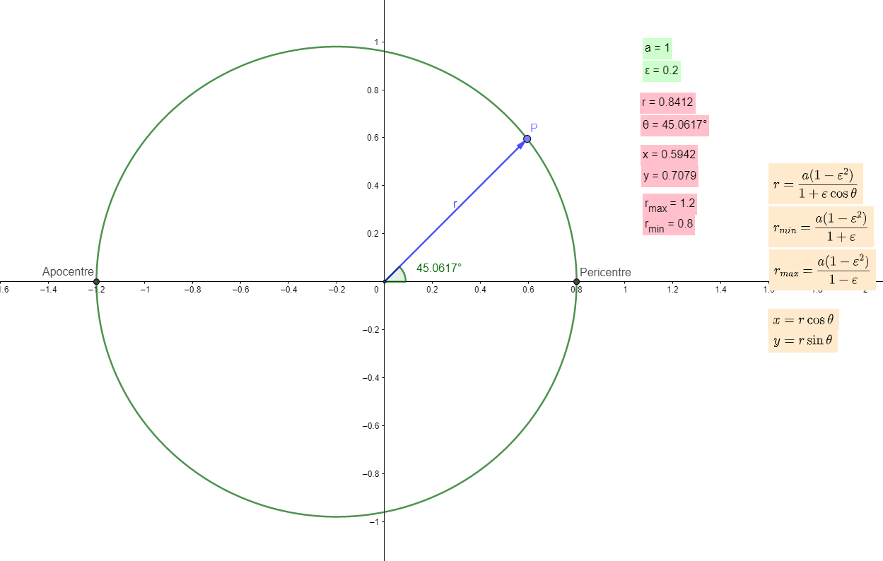
Most orbits are elliptical, although some are relatively close to circular such as the earth-sun and geosynchronous satellites, none are exactly perfect and will drift over time due to orbital perturbations, the following equation can plot a circle, ellipse, parabola or hyperbola depending on the eccentricity value, if you are not familar eccentricity is a unitless value that determines the shape of an orbit, 0 is a circle, between 0 and 1 is an ellipse, exactly 1 is a parabola and greater than 1 is a hyperbola.
To plot in polar form the equation is:
$$ r = \frac{a(1-\varepsilon^2)}{1+\varepsilon \cos \theta} $$
Where a is the semi-major axis of the ellipse (the radius from the focal point) and ε (epsilon) is the eccentricity of the orbit, this can be converted to rectangular form with:
$$ x = r \cos \theta $$
$$ y = r \sin \theta $$
The maximum and minimum distance from the focal point can be calculated with:
$$r_{min} = \frac{a(1-\varepsilon^2)}{1+\varepsilon}$$
$$r_{max} = \frac{a(1-\varepsilon^2)}{1-\varepsilon}$$
An example of the results can be seen below:
Rectangular form
If you’d rather plot directly in rectangular rather than polar you can use this equation:
$$ \frac{(x+F_1)^2}{a^2} + \frac{y^2}{b^2}=1 $$
Where b is the semi-minor axis, and F1 is one of the two focal points, in this case the one on the right is chosen to match up with the polar equation which uses the right focal point also, the semi-minor axis can be calculated with:
$$ b = a \sqrt{1- \varepsilon^2} $$
And for the focal point:
$$ F_1 = \sqrt{a^2 – b^2} $$
Since it’s centred on the focal point F1, the centre of the ellipse is at (-F1,0) whilst F2 is at (-2*F1,0), it’s important to note that this equation does not work with an eccentricity equal or above 1.
Alternative equation
The alternative form given in the Wikipedia article is somewhat more complicated but yields the same results, in order for this to work you need to know the velocity at periapsis.
To calculate the velocity you can use the vis-viva equation, using the distance to periapsis:
$$v =\sqrt{\mu \frac{2}{r_{min}}-\frac{1}{a}}$$
Where μ is the gravitational parameter:
$$\mu = GM$$
For example for earth:
$$v =\sqrt{1.327184555 \times 10^{20} \frac{2}{1.47095 \times 10^{11}}-\frac{1}{1.49598023 \times ^{11}}} = \approx 30287.94 \text{m}/\text{s}$$
The equation to plot the orbit is:
$$r = \frac{\ell^2}{m^2\mu}\frac{1}{1+\varepsilon\cos{\theta}}$$
Where m is the mass of the secondary body and the angular momentum ℓ is:
$$\ell = m v r_{min}$$